The Leap from Classic to Quantum

Classic Deterministic Systems

definition

If $f:\mathbb{R}^n\rightarrow\mathbb{R}^n$ is a transformation and $\cdots, \boldsymbol{x}_t, \boldsymbol{x}_{t+1}, \boldsymbol{x}_{t+2}, \cdots$ is a sequence of vectors in $\mathbb{R}^n$ such that $\boldsymbol{x}_{t+1}=f(\boldsymbol{x}_{t})$, then we say that $f$ and sequence $\cdots, \boldsymbol{x}_t, \boldsymbol{x}_{t+1}, \boldsymbol{x}_{t+2}, \cdots$ make up a discrete dynamical system, where function $f$ is called dynamics and vectors $\{\boldsymbol{x}_t\}$ are called states.

Figure 1.1: Classic billiards

example:classic-billiards

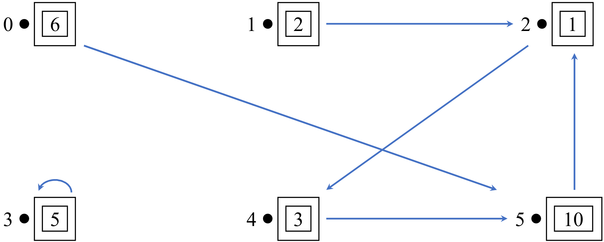
Let's consider a simple system described by a simple (unweighted) directed graph together with some toy marbles. There be $6$ vertices in a graph and a total of $27$ marbles. We might place $6$ marbles on vertex $0$, $2$ marbles on vertex $1$, and the rest as described by Figure 1.1.

We shall denote its deterministic state as $\boldsymbol{x}=[6,2,1,5,3,10]^{\top}$, and its dynamics as a Boolean adjacency matrix $\mathbf{M}= \begin{bmatrix} 0 & 0 & 0 & 0 & 0 & 0 \\ 0 & 0 & 0 & 0 & 0 & 0 \\ 0 & 1 & 0 & 0 & 0 & 1 \\ 0 & 0 & 0 & 1 & 0 & 0 \\ 0 & 0 & 1 & 0 & 0 & 0 \\ 1 & 0 & 0 & 0 & 1 & 0 \end{bmatrix}$ where $\mathbf{M}(i,j)=1$ if and only if there is an arrow from vertex $j$ to vertex $i$.

The state evolvement can be represented as matrix multiplication: $\boldsymbol{x}_{t+1}=f(\boldsymbol{x}_{i})=\mathbf{M}\boldsymbol{x}_{t}$

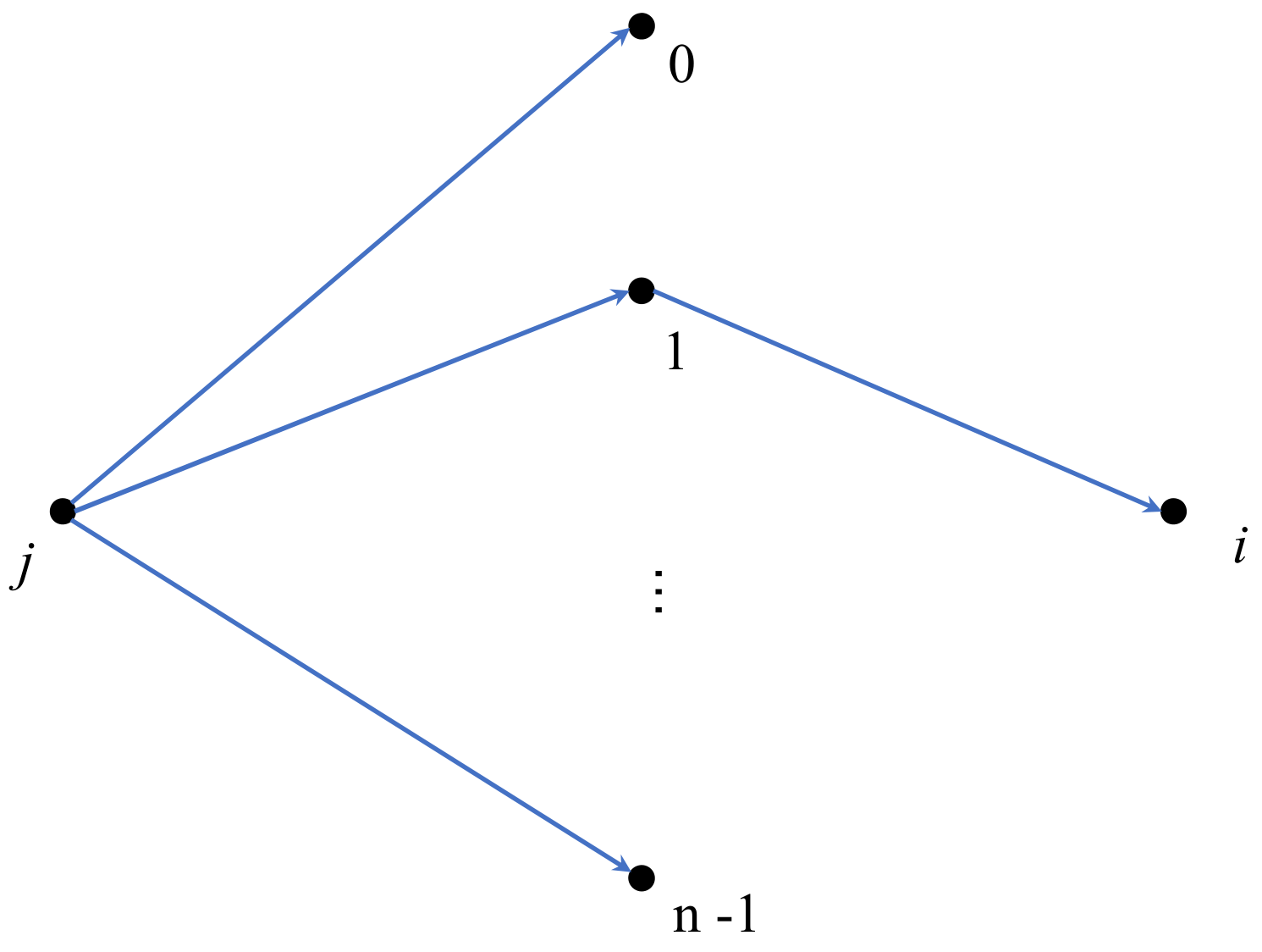
The multiple step dynamics can be written as Boolean matrix multiplication: $\mathbf{M}^2(i,j)=\bigvee_{k=0}^{n-1}\mathbf{M}(i,k)\wedge\mathbf{M}(k,j)$ where $\vee$ and $\wedge$ represent Boolean "OR" and "AND" operators, and $\mathbf{M}^2(i,j)=1$ if and only if there is a path of length 2 from vertex $j$ to vertex $i$ as shown in Figure 1.2.

Figure 1.2: multiple step dynamics

Probabilistic Systems

The state of a probabilistic system is composed of probabilistic entries, and the sum of all entries is $1$.

example: probabilistic system

$\boldsymbol{x}=\left[\frac{1}{5}, \frac{3}{10}, \frac{1}{2}\right]^{\top}\nonumber$

• one-fifth chance that the marble is on vertex 0;

• three-tenths chance that the marble is on vertex 1;

• half chance that the marble is on vertex 2.

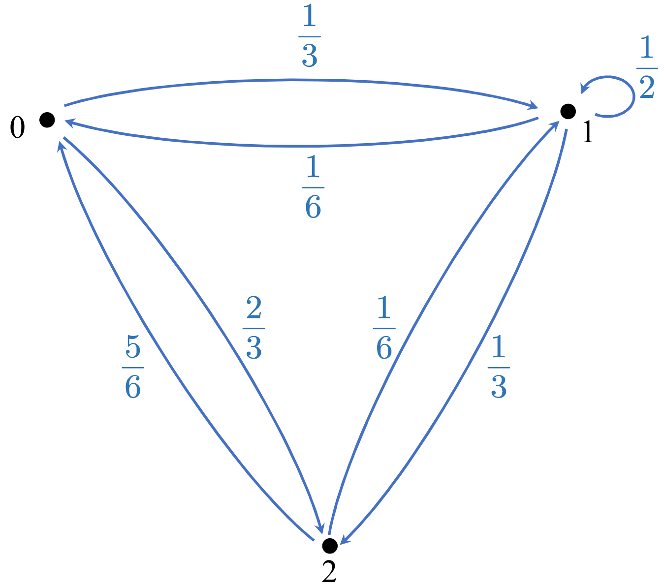
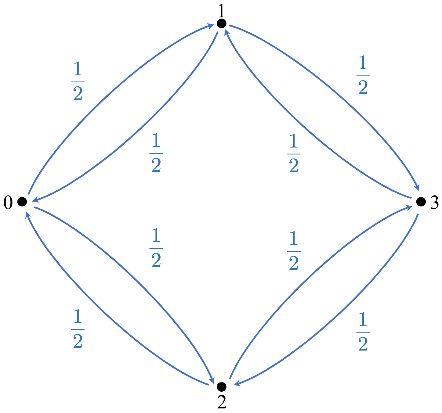
The dynamics of a probabilistic system is described by a directed (probabilistic) weighted graph, where several arrows shooting out of each vertex with real numbers between 0 and 1 as weights as shown in Figure 1.3. The corresponding matrix is called doubly stochastic matrix, which has the following two properties:

• The column sum, i.e., the sum of all weights leaving a vertex, is $1$;

• The row sum, i.e., the sum of all weights entering a vertex, is $1$.

Figure 1.3: probabilistic system

The state evolvement. If we have $\boldsymbol{x}_t$ expressing the probability of the position of the marble at time $t$ and $\mathbf{M}$ expressing the probability of the way the marble moves around, then $\boldsymbol{x}_{t+1}=\mathbf{M}\boldsymbol{x}_t$ is expressing the probability of the marble's location at time $t + 1$.

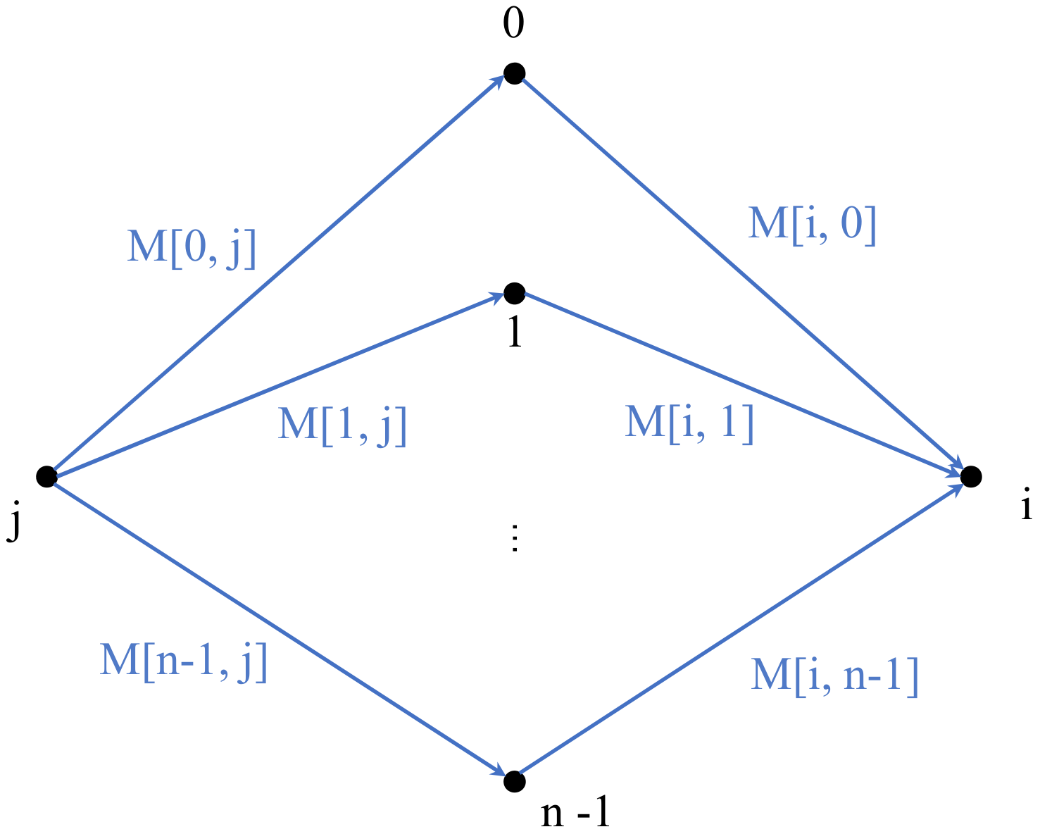
The multiple step dynamics of probabilistic system is formulated with matrix multiplication with probability entries (a.k.a., normal matrix multiplication). Figure 1.4 shows an example of the 2-step dynamics.

Figure 1.4:The 2-step dynamics in the probabilistic system

Figure 1.5: stochastic-billiard

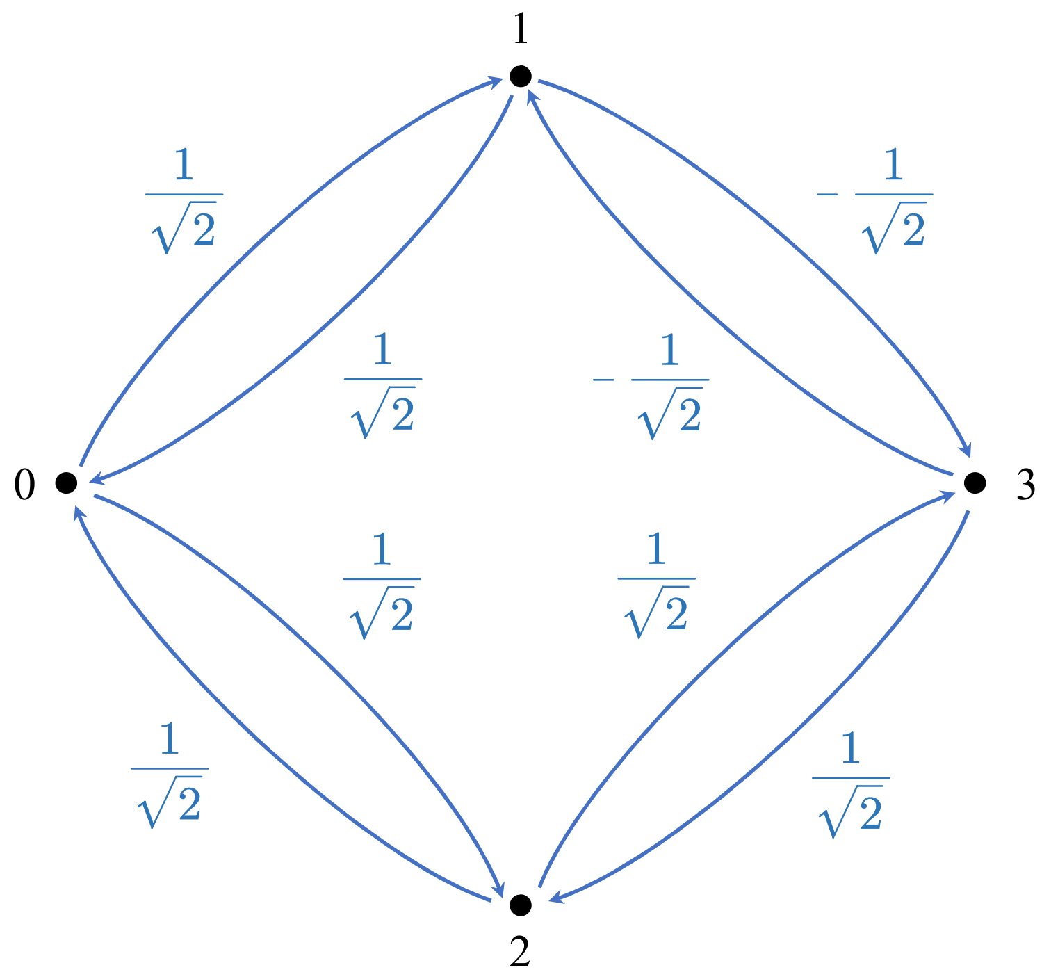
example: stochastic-billiard

Consider a stochastic billiard with dynamics shown in Figure 1.5 and initial state $\boldsymbol{x}_{0}$, its state evolvement procedure exhibits periodic cycles as follows: $\begin{aligned}\boldsymbol{x}_{0}=\begin{bmatrix}1 & 0 & 0 & 0\end{bmatrix}^{\top}&\stackrel{\mathbf{M}}{\longmapsto}{\color{red}\boldsymbol{x}_{1}}=\begin{bmatrix}0 & \frac{1}{2} & \frac{1}{2} & 0\end{bmatrix}^{\top}\stackrel{\mathbf{M}}{\longmapsto}{\color{blue}\boldsymbol{x}_{2}}=\begin{bmatrix}\frac{1}{2} & 0 & 0 & \frac{1}{2}\end{bmatrix}^{\top}\\&\stackrel{\mathbf{M}}{\longmapsto}\boldsymbol{x}_{3}={\color{red}\boldsymbol{x}_{1}}\stackrel{\mathbf{M}}{\longmapsto}\boldsymbol{x}_{4}={\color{blue}\boldsymbol{x}_{2}}\stackrel{\mathbf{M}}{\longmapsto}\cdots\end{aligned}$

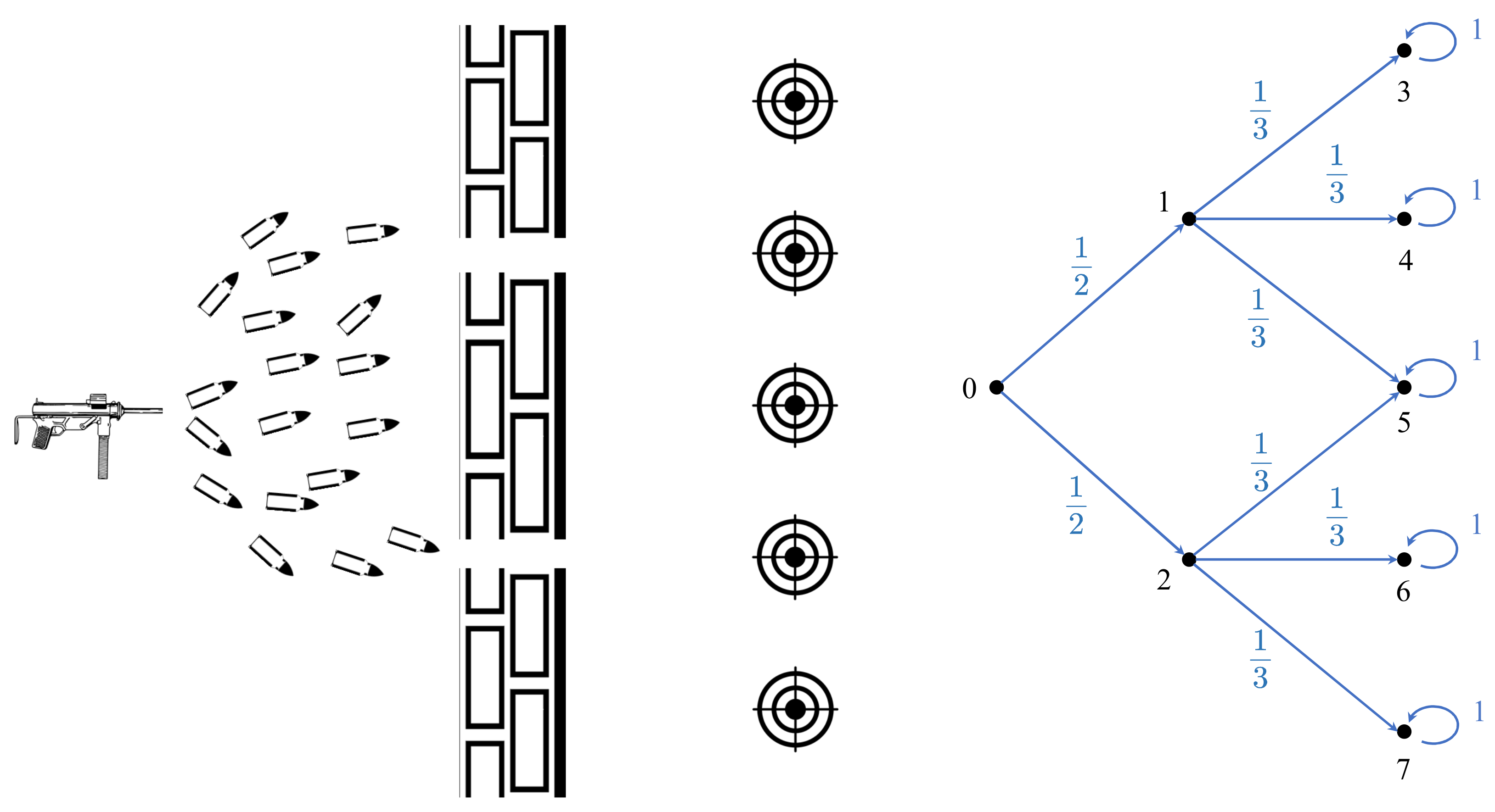
Figure 1.6: probabilistic-double-silt

example:probabilistic-double-silt

Assume a virtual double silt experiment as shown in Figure 1.6. The bullets are fired from the machine-gun, pass through two narrow slits in the wall, and eventually land on the targets behind the wall. Its dynamics matrix can be formulated as $\mathbf{M}=\begin{bmatrix} 0 & 0 & 0 & 0 & 0 & 0 & 0 & 0\\[4pt]\frac{1}{2} & 0 & 0 & 0 & 0 & 0 & 0 & 0\\[4pt]\frac{1}{2} & 0 & 0 & 0 & 0 & 0 & 0 & 0\\[4pt]0 & \frac{1}{3} & 0 & 0 & 0 & 0 & 0 & 0\\[4pt]0 & \frac{1}{3} & 0 & 0 & 0 & 0 & 0 & 0\\[4pt]0 & \frac{1}{3} & \frac{1}{3} & 0 & 0 & 0 & 0 & 0\\[4pt]0 & 0 & \frac{1}{3} & 0 & 0 & 0 & 0 & 0\\[4pt]0 & 0 & \frac{1}{3} & 0 & 0 & 0 & 0 & 0\\[4pt]\end{bmatrix}\nonumber$ and accordingly, its $2$-step dynamics can be computed by matrix multiplication: $\mathbf{M}^2=\mathbf{M}\times \mathbf{M}=\begin{bmatrix}0 & 0 & 0 & 0 & 0 & 0 & 0 & 0\\[4pt]0 & 0 & 0 & 0 & 0 & 0 & 0 & 0\\[4pt]0 & 0 & 0 & 0 & 0 & 0 & 0 & 0\\[4pt]\frac{1}{6} & \frac{1}{3} & 0 & 1 & 0 & 0 & 0 & 0\\[4pt]\frac{1}{6} & \frac{1}{3} & 0 & 0 & 1 & 0 & 0 & 0\\[4pt]\color{red}\frac{1}{3} & \frac{1}{3} & 0 & 0 & 1 & 0 & 0\\[4pt]\frac{1}{6} & 0 & \frac{1}{3} & 0 & 0 & 0 & 1 & 0\\[4pt]\frac{1}{6} & 0 & \frac{1}{3} & 0 & 0 & 0 & 0 & 1\\[4pt]\end{bmatrix}\nonumber$ Hence, given an initial state $\boldsymbol{x}_0=\begin{bmatrix} 1 & 0 & 0 & 0 & 0 & 0 & 0 & 0 \end{bmatrix}^{\top}$, its $2$-step transition state $\boldsymbol{x}_2=\mathbf{M}^2\boldsymbol{x}_0=\begin{bmatrix} 0 & 0 & 0 & \frac{1}{6} & \frac{1}{6} & \color{red}\frac{1}{3} & \frac{1}{6} & \frac{1}{6} \end{bmatrix}^{\top}$.

Note that the probability of the bullets landing on the middle target is the largest, i.e., $\color{red}\frac{1}{3}$. This is consistent with our knowledge because both routes can reach this target, meaning a summation of probabilities.

Quantum Systems

The state of a quantum system is composed of quantum entries (complex values), whose modulus square represents the probability, and the sum of modulus squared of all entries is $1$.

example:quantum-state

Consider a complex vector $\boldsymbol{x}=\left[\frac{1}{\sqrt{3}}, \frac{2i}{\sqrt{15}}, \sqrt{\frac{2}{5}}\right]^{\top}$, since $\boldsymbol{x}^{\dagger}\boldsymbol{x}=\frac{1}{3}+\frac{4}{15}+\frac{2}{5}=1$, it is a qualified state vector of a quantum system.

The dynamics of a quantum system also has two representations. One is the graph form, which can be described by a directed (complex) weighted graph. The other is the matrix form, which corresponds to a special unitary matrix whose modulus square is a doubly stochastic matrix as exemplified in Figure 1.7.

Figure 1.7: quantum-system

Table below gives a detailed comparison of three systems in terms their states and dynamics. In particular, the dynamics is represented in two different forms, which are graph (Gra.) and matrix (Mat.), respectively.

	Classic Deterministic System	Probabilistic System	Quantum System
State	$\boldsymbol{x}=[x_1, x_2, x_3]^{\top}$, $x_i\in\mathbb{N}$	$\boldsymbol{x}=[p_1, p_2, p_3]^{\top}$, $x_i\in[0,1], \sum_i p_i=1$	$\boldsymbol{x}=[c_1, c_2, c_3]^{\top}$,$c_i\in\mathbb{C}, \sum_i$
Dynamics (Gra.)	Directed unweighted graph	Directed (probabilistic) weighted graph	Directed (complex) weighted graph
Dynamics (Mat.)	Boolean adjacency matrix	Doubly stochastic matrix	Unitary matrix whose modulus squares is a doubly stochastic matrix

The state evolvement is formulated as matrix multiplication $\boldsymbol{x}_{t+1}=\mathbf{M}\boldsymbol{x}_{t}$.

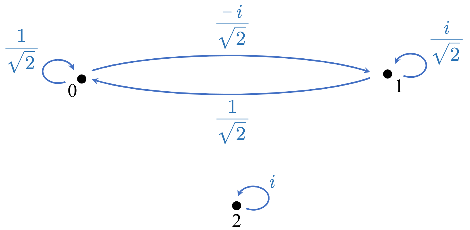
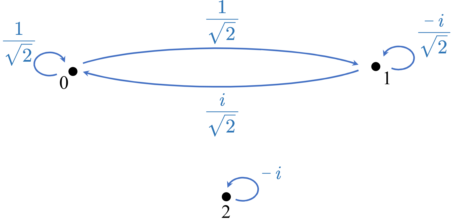
The forward dynamics and backward dynamics can be represented as a matrix $\mathbf{M}$ and its adjoint $\mathbf{M}^{\dagger}$ as shown in the following Table. This means that if you perform some operation $\boldsymbol{x}\mapsto\mathbf{M}\boldsymbol{x}$ and then "undo" the operation $\mathbf{M}^{\dagger}\mathbf{M}\boldsymbol{x}=\mathbf{I}\boldsymbol{x}=\boldsymbol{x}$, you will find yourself (with probability 1) in the same state with which you began.

	Dynamics graph	Dynamics Matrix
Forward dynamics		$\mathbf{M}=\begin{bmatrix}\frac{1}{\sqrt{2}} & \frac{1}{\sqrt{2}} & 0\\[8pt]\frac{-i}{\sqrt{2}} & \frac{i}{\sqrt{2}} & 0\\[8pt]0 & 0 & i\\[4pt]\end{bmatrix}$
Backward dynamics		$\mathbf{M}=\begin{bmatrix}\frac{1}{\sqrt{2}} & \frac{i}{\sqrt{2}} & 0\\[8pt]\frac{1}{\sqrt{2}} & \frac{-i}{\sqrt{2}} & 0\\[8pt]0 & 0 & -i\\[4pt]\end{bmatrix}$

Figure 1.8: quantum billiard

example

Consider a quantum billiard with dynamics shown in Figure 1.8 and initial state $\boldsymbol{x}_{0}$, its state evolvement procedure exhibits periodic cycles as follows: $\begin{aligned}\boldsymbol{x}_{0}=\begin{bmatrix}1 & 0 & 0 & 0\end{bmatrix}^{\top}&\stackrel{\mathbf{M}}{\longmapsto}{\color{black}\boldsymbol{x}_{1}}=\begin{bmatrix}0 & \frac{1}{\sqrt{2}} & \frac{1}{\sqrt{2}} & 0\end{bmatrix}^{\top}\\&\stackrel{\mathbf{M}}{\longmapsto}{\color{black}\boldsymbol{x}_{2}}={\color{red}\boldsymbol{x}_{0}}\stackrel{\mathbf{M}}{\longmapsto}\boldsymbol{x}_{3}={\color{blue}\boldsymbol{x}_{1}}\stackrel{\mathbf{M}}{\longmapsto}\cdots\end{aligned}$

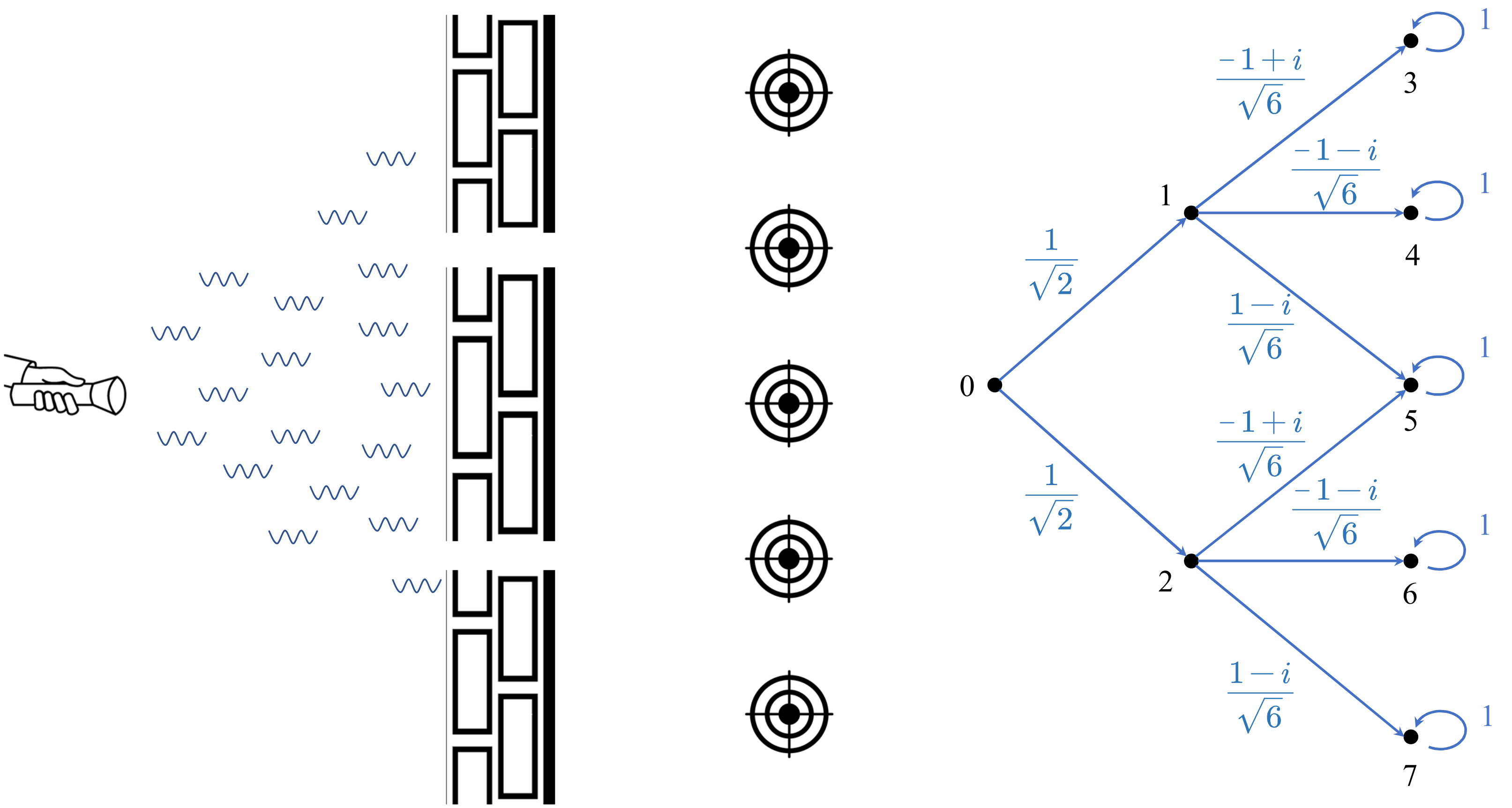
Figure 1.9: Double slit experiment

example

Given a double silt experiment as shown in Figure 1.9. The photons are ejected from the flashlight, pass through two narrow slits in the wall, and eventually land on the screens behind the wall. Its 1-step and 2-step dynamics matrices are respectively $\mathbf{M}=\begin{bmatrix} 0 & 0 & 0 & 0 & 0 & 0 & 0 & 0\\[8pt] \frac{1}{\sqrt{2}} & 0 & 0 & 0 & 0 & 0 & 0 & 0\\[8pt] \frac{1}{\sqrt{2}} & 0 & 0 & 0 & 0 & 0 & 0 & 0\\[8pt] 0 & \frac{-1+i}{\sqrt{6}} & 0 & 1 & 0 & 0 & 0 & 0\\[8pt] 0 & \frac{-1-i}{\sqrt{6}} & 0 & 0 & 1 & 0 & 0 & 0\\[8pt] 0 & \frac{1-i}{\sqrt{6}} & \frac{-1+i}{\sqrt{6}} & 0 & 0 & 1 & 0 & 0\\[8pt] 0 & 0 & \frac{-1-i}{\sqrt{6}} & 0 & 0 & 0 & 1 & 0\\[8pt] 0 & 0 & \frac{1-i}{\sqrt{6}} & 0 & 0 & 0 & 0 & 1\\[8pt] \end{bmatrix}\nonumber\mapsto \mathbf{M}^2=\begin{bmatrix} 0 & 0 & 0 & 0 & 0 & 0 & 0 & 0\\[8pt] 0 & 0 & 0 & 0 & 0 & 0 & 0 & 0\\[8pt] 0 & 0 & 0 & 0 & 0 & 0 & 0 & 0\\[8pt] \frac{-1+i}{\sqrt{12}} & \frac{-1+i}{\sqrt{6}} & 0 & 1 & 0 & 0 & 0 & 0\\[8pt] \frac{-1-i}{\sqrt{12}} & \frac{-1-i}{\sqrt{6}} & 0 & 0 & 1 & 0 & 0 & 0\\[8pt] \color{red}{0} & \frac{1-i}{\sqrt{6}} & \frac{-1+i}{\sqrt{6}} & 0 & 0 & 1 & 0 & 0\\[8pt] \frac{-1-i}{\sqrt{12}} & 0 & \frac{-1-i}{\sqrt{6}} & 0 & 0 & 0 & 1 & 0\\[8pt] \frac{-1+i}{\sqrt{12}} & 0 & \frac{1-i}{\sqrt{6}} & 0 & 0 & 0 & 0 & 1\\[8pt] \end{bmatrix}\nonumber$ Note that $\mathbf{M}(5,0)=\frac{1}{\sqrt{2}}(\frac{1-i}{\sqrt{6}})+\frac{1}{\sqrt{2}}(\frac{-1+i}{\sqrt{6}})=\frac{1-i}{\sqrt{12}}+\frac{-1+i}{\sqrt{12}}=\frac{0}{\sqrt{12}}=\color{red}{0}$, which is called interference phenomenon.

Superposition. Let the state of the system be given by $\boldsymbol{x}= [c_0, c_1, \cdots ,c_{n−1}]^{\top}\in\mathbb{C}^n$. It is incorrect to say that the probability of the photon's being in position $k$ is $|c_k|^2$. Rather, to be in state $\boldsymbol{x}$ means that the particle is in some sense in all positions simultaneously. The photon passes through the top slit and the bottom slit simultaneously, and when it exits both slits, it can cancel itself out. A photon is not in a single position, rather it is in many positions, a superposition.

Measurement and collapse. The reason we see particles in one particular position is because we have performed a measurement. When we measure something at the quantum level, the quantum object that we have measured is no longer in a superposition of states, rather it collapses to a single classical state. So we have to redefine what the state of a quantum system is: a system is in state $\boldsymbol{x}$ means that after measuring it, it will be found in position $i$ with probability $|c_i|^2$.

Power of quantum computing. It is exactly this superposition of states that is the real power behind quantum computing. Classical computers are in one state at every moment. Imagine putting a computer in many different classical states simultaneously and then processing with all the states at once. This is the ultimate in parallel processing!