Introduction and Complex Number

Introduction to Quantum Computing

A brief history

Quantum Mechanics as a branch of physics began with a set of scientific discoveries in the late $19$th Century and has been in active development ever since. Most people will point to the 1980s as the start of physicists actively looking at computing with quantum systems¹:

• 1982: History of quantum computing starts with Richard Feynman lectures on the potential advantages of computing with quantum systems.

• 1985: David Deutsch publishes the idea of a "universal quantum computer".

• 1994: Peter Shor presents an algorithm that can efficiently find the factors of large numbers, significantly outperforming the best classical algorithm and theoretically putting the underpinning of modern encryption at risk (referred to now as Shor's algorithm).

• 1996: Lov Grover presents an algorithm for quantum computers that would be more efficient for searching databases (referred to now as Grove's search algorithm).

• 1996: Seth Lloyd proposes a quantum algorithm which can simulate quantum-mechanical systems.

• 1999: D-Wave Systems founded by Geordie Rose.

• 2000: Eddie Farhi at MIT develops idea for adiabatic quantum computing.

• 2001: IBM and Stanford University publish the first implementation of Shor's algorithm, factoring 15 into its prime factors on a 7-qubit processor.

• 2010: D-Wave One: first commercial quantum computer released (annealer).

• 2016: IBM makes quantum computing available on IBM Cloud.

• 2019: Google claims the achievement of quantum supremacy. Quantum Supremacy was termed by John Preskill in 2012 to describe when quantum systems could perform tasks surpassing those in the classical world.

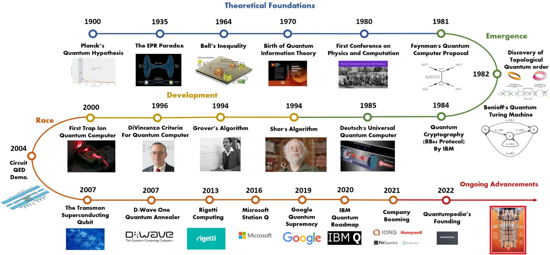
A more complete history comes from the quantumpedia², where the development of quantum computing is divided into five distinct periods Figure 1.1:

Figure 1.1: history

Prof. Andrew Chi-Chih Yao's Talk in Micius Salon

Prof. Yao gave a talk entitled "The Advent of Quantum Computing" in Micius Salon in 2018³. Here are some key points:

• Two key topics: (1) what is the nature of quantum computer?; and (2) where does quantum computer gets its power from?

• The particle-wave duality plays the starting role in making it possible for us to do quantum computing faster than classic computing under certain circumstances

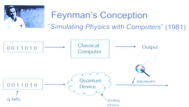
• Richard Feynman's question: can quantum physics be simulated efficiently? Answer: unlikely by a classic computer, but hopefully by a quantum computer.

• The comparison of classic computer and quantum computers (Figure 1.2). Classic computers manipulate classic bits $0110\cdots$ with Boolean operations in $\{0,1\}^n$, while quantum computers manipulate quantum bits $\ket{0101\cdots}$ with "rotations" in $\mathbb{C}^{2^n}$

Figure 1.2: The comparison of classic and quantum computers

• The parallel superposition is brought by the fact that each quantum bit represents not a single state, but a "probabilistic distribution" of state. Parallelism could speed up computational tasks.

• quantum parallelism is only a metaphor, subtle and restricted, not equivalent to a parallel computer with many processors.

Complex Numbers

The original motivation for the introduction of complex numbers was seeking solutions of polynomial equations. Here is the simplest example: $x^2+1=0$ Obviously, we cannot find its solution in the set of real numbers. To solve this problem, Mathematics introduces following definitions.

Definitions

definition

An imaginary number is a real number multiplied by the imaginary unit $i$, which is defined by its property $i^2 = −1$ or $i=\sqrt{-1}$.

definition

A complex number is a hybrid entity which adds a real number with an imaginary number, for instance, $c=a+b\times i=a+bi$ where $a$, $b$ are two real numbers, $a$ is called the real part of $c$, whereas $b$ is its imaginary part. The set of all complex numbers will be denoted as $\mathbb{C}$. When the $\times$ is understood, we shall omit it.

proposition

Every polynomial equation of one variable with complex coefficients has a complex solution.

The Algebra of Complex Numbers

definition

Ordered pair representation defines a complex number as an ordered pair of reals: $c=a+bi\mapsto (a, b)$

Hence, ordinary real numbers can be identified with pairs $(a, 0)$ $a\mapsto (a, 0)$ whereas imaginary numbers can be identified with pairs $(0, b)$. In particular, $i\mapsto (0, 1)$

The four arithmetic operations between two complex numbers can be expressed as:

• Addition: $c_1+c_2=(a_1, b_1)+(a_2, b_2) = (a_1+a_2, b_1+b_2)$

• Subtraction: $c_1-c_2=(a_1, b_1)-(a_2, b_2) = (a_1-a_2, b_1-b_2)$

• Multiplication: $c_1\times c_2=(a_1, b_1)\times (a_2, b_2) = (a_1a_2-b_1b_2, a_1b_2+a_2b_1)$

• Subdivision: $\frac{c_1}{c_2}=\frac{(a_1, b_1)}{(a_2, b_2)}=(\frac{a_1a_2+b_1b_2}{a_2^2+b_2^2}, \frac{a_2b_1-a_1b_2}{a_2^2+b_2^2})$

With the addition and multiplication operations, we can re-write a complex number as $c = a+bi = (a, b) = (a, 0) + (0, b) = (a, 0) + (b, 0)\times (0, 1)$ and from the denominator in the quotient formula in Subdivision, we can define the modulus of a complex number as: $|c|=|a+bi|=+\sqrt{a^2+b^2}$ which has two useful properties:

• Property 1: $\forall c_1, c_2\in\mathbb{C}, |c_1||c_2|=|c_1c_2|$.

• Property 2: $\forall c_1, c_2\in\mathbb{C}, |c_1+c_2|\leq|c_1|+|c_2|$.

where the second property is also called triangular inequality of modulus operation.

Based on the above basic operations, it is easy to verify that complex numbers have the following algebraic properties:

• Addition has an identity called additive identity: $(0, 0)$, such that $\forall c\in\mathbb{C}, c+(0, 0)=c$

• Multiplication has an identity called multiplicative identity: $(1, 0)$, such that $\forall c\in\mathbb{C}, c\times(1, 0)=(1, 0)\times c=c$

• Both addition and multiplication are commutative: $\left\{ \begin{aligned} c_1+c_2&=c_2+c_1\\ c_1\times c_2&=c_2\times c_1 \end{aligned} \right.$

• Both addition and multiplication are associative: $\left\{ \begin{aligned} (c_1+c_2)+c_3&=c_1+(c_2+c_3)\\ (c_1\times c_2)\times c_3&=c_1\times (c_2\times c_3) \end{aligned} \right.$

• Multiplication distributes with respect to addition: $c_1\times(c_2+c_3)=c_1\times c_2+c_1\times c_3$

• Subtraction is defined everywhere.

• Division is defined everywhere except when the divisor is zero.

Besides basic arithmetic operations and modulus operation, complex numbers have a unique operation called conjugation. If $c=a+bi$ is an arbitrary complex number, then the conjugate of $c$ is $\overline{c}=a-bi$. Two numbers related by conjugation are said to be complex conjugates of each other. The conjugation operation has several basic properties:

• Property 1: Conjugate respects addition $\overline{c_1+c_2}=\overline{c_1}+\overline{c_2}$.

• Property 2: Conjugate respects multiplication $\overline{c_1\times c_2}=\overline{c_1}\times \overline{c_2}$.

• Property 3: Conjugate $c\mapsto \overline{c}$ is bijective.

• Property 4: The modulus squared of a complex number is obtained by multiplying the number with its conjugate $c\times \overline{c}=|c|^2$.

The Geometry of Complex Numbers

definition

The complex plane is the plane formed by the complex numbers, with a Cartesian coordinate system such that the horizontal x-axis, called the real axis, is formed by the real numbers, and the vertical y-axis, called the imaginary axis, is formed by the imaginary numbers.

In the complex plane (Figure fig:complex-plane), we can easily find that the modulus is nothing more than the length of the vector. Indeed, the length of a vector, via Pythagoras' theorem, is the square root of the sum of the squares of its edges, which is precisely the modulus, as defined in the previous section.

The complex plane

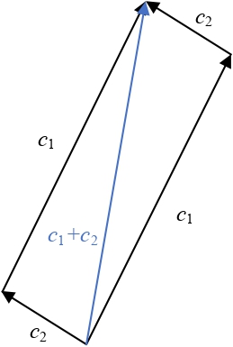
Next comes addition: vectors can be added using the so-called parallelogram rule illustrated by Figure parallelogram-rule-addition. In words, draw the parallelogram whose parallel edges are the two vectors to be added; their sum is the diagonal.

The parallelogram rule addition

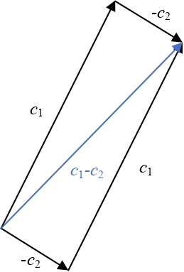
Subtraction too has a clear geometric meaning: subtracting $c_2$ from $c_1$ is the same as adding the negation of $c_2$, i.e., $-c_2$, to $c_1$ (Figure parallelogram-rule-subtraction).

The parallelogram rule subtraction

To give a simple geometrical meaning to multiplication, we need to develop yet another characterization of complex numbers.

definition

The polar coordinate system is a two-dimensional coordinate system in which each point on a plane is determined by a distance $\rho$ from a reference point and an angle $\theta$ from a reference direction.

Similar to the previous Cartesian representation $(a, b)$, the polar representation $(\rho, \theta)$ is capable to uniquely determine a complex number because these two representations can be mutually converted:

representation 1

2 $(a, b)\mapsto (\rho, \theta)$ where $\rho$ is the modulus $\rho=\sqrt{a^2+b^2}$ and $\theta$ is also easy, via trigonometry $\theta=\tan^{-1}\Bigg(\frac{b}{a}\Bigg)$

representation 2

$(\rho, \theta)\mapsto (a, b)$ where $a$ is the real part $a = \rho\cos(\theta)$ and $b$ is the imaginary part $b = \rho\sin(\theta)$

In physics and engineering, angle $\theta$ is also known as phase and distance $\rho$ is also known as magnitude. Hence, we have another definition of a complex number

definition

A complex number is a magnitude and a phase.

We are now ready for multiplication: given two complex numbers in polar coordinates, $c_1=(\rho_1, \theta_1)$ and $c_2=(\rho_2, \theta_2)$, their product can be obtained by simply multiplying their magnitude and adding their phase: $c_1\times c_2=(\rho_1, \theta_1)\times (\rho_2, \theta_2)=(\rho_1\rho_2, \theta_1+\theta_2)$

Now that we are armed with a geometric way of looking at multiplication, we can tackle division as well. After all, division is nothing more than the inverse operation of multiplication: $\frac{c_1}{c_2}=\Bigg(\frac{\rho_1}{\rho_2}, \theta_1-\theta_2\Bigg)$

On this basis, we can further derive fast $n$-order power and root calculations about a complex number $c=(\rho, \theta)$ $c^n=(\rho^n, n\theta)$ and $c^{\frac{1}{n}}=\Bigg(\rho^{\frac{1}{n}}, \frac{1}{n}(\theta+k2\pi)\Bigg),\ \textrm{where}\ k=0,1,\cdots,n-1$

Footnotes

1. history of quantum computing ↩

2. a brief history of quantum computing ↩

3. bilibili ↩