Complex Vector Space

Complex Vector Space

definition

A complex vector space is a nonempty set $\mathbb{V}$, whose elements we shall call vectors, with three operations

• Addition: $+$: $\mathbb{V}\times \mathbb{V}\rightarrow \mathbb{V}$

• Negation: $-$: $\mathbb{V}\rightarrow \mathbb{V}$

• Scalar multiplication: $\cdot$: $\mathbb{C}\times \mathbb{V}\rightarrow \mathbb{V}$

and a distinguished element called the zero vector $\boldsymbol{0}\in \mathbb{V}$ in the set. These operations and zero must satisfy the following properties: $\forall \boldsymbol{v, w, x}\in \mathbb{V}$ and for all $c, c_1, c_2\in\mathbb{C}$,

i. Commutativity of addition: $\boldsymbol{v}+\boldsymbol{w} = \boldsymbol{w}+\boldsymbol{v}$,

ii. Associativity of addition: $(\boldsymbol{v}+\boldsymbol{w}) + \boldsymbol{x} = \boldsymbol{v} + (\boldsymbol{w}+\boldsymbol{x})$,

iii. Additive identity: $\boldsymbol{v} + \boldsymbol{0} = \boldsymbol{v} = \boldsymbol{0} + \boldsymbol{v}$,

iv. Additive inverse: $\boldsymbol{v} + (-\boldsymbol{v}) = \boldsymbol{0} = (-\boldsymbol{v}) + \boldsymbol{v}$,

v. Multiplication identity: $1\cdot \boldsymbol{v}=\boldsymbol{v}$,

vi. Scalar multiplication distributes over addition: $c\cdot(\boldsymbol{v}+\boldsymbol{w})=c\cdot \boldsymbol{v}+c\cdot\boldsymbol{w}$,

vii. Scalar multiplication distributes over complex addition: $(c_1+c_2)\cdot\boldsymbol{v}=c_1\cdot \boldsymbol{v}+c_2\cdot\boldsymbol{v}$,

example

ex:n-dim-vector-space $\mathbb{C}^n$, the set of vectors of length $n$ with complex entries, is a complex vector space.

example

ex:nn-dim-vector-space $\mathbb{C}^{m\times n}$, the set of all $m$-by-$n$ matrices (two-dimensional arrays) with complex entries, is a complex vector space.

Unary Operations

Three unary operations for $\forall \mathbf{A}\in\mathbb{C}^{m\times n}$

• Transpose: $\mathbf{A}^{\top}\in\mathbb{C}^{n\times m} \textrm{\ \ such that\ \ } \mathbf{A}^{\top}(j,k)=\mathbf{A}^{\top}(k,j)$

• Conjugate: $\overline{\mathbf{A}}\in\mathbb{C}^{m\times n} \textrm{\ \ such that\ \ } \overline{\mathbf{A}}(j,k)=\overline{\mathbf{A}(j,k)}$

• Ajoint: $\mathbf{A}^{\dagger}\in\mathbb{C}^{n\times m} \textrm{\ \ such that\ \ } \mathbf{A}^{\dagger}(j,k)=\overline{\mathbf{A}(k,j)}$

property

$\forall c\in \mathbb{C}$ and $\mathbf{A}, \mathbf{B}\in\mathbb{C}^{m\times n}$

• Transpose is idempotent: $(\mathbf{A}^{\top})^{\top}=\mathbf{A}$

• Transpose respects addition: $(\mathbf{A}+\mathbf{B})^{\top}=\mathbf{A}^{\top}+\mathbf{B}^{\top}$

• Transpose respects scalar multiplication: $(c\cdot \mathbf{A})^{\top}=c\cdot \mathbf{A}^{\top}$

property

$\forall c\in \mathbb{C}$ and $\mathbf{A}, \mathbf{B}\in\mathbb{C}^{m\times n}$

• Conjugate is idempotent: $\overline{\overline{\mathbf{A}}}=\mathbf{A}$

• Conjugate respects addition: $\overline{\mathbf{A}+\mathbf{B}}=\overline{\mathbf{A}}+\overline{\mathbf{B}}$

• Conjugate respects scalar multiplication: $\overline{c\cdot \mathbf{A}}=\overline{c}\cdot \overline{\mathbf{A}}$

property

$\forall c\in \mathbb{C}$ and $\mathbf{A}, \mathbf{B}\in\mathbb{C}^{m\times n}$

• Adjoint is idempotent: ${(\mathbf{A}^{\dagger})}^{\dagger}=\mathbf{A}$

• Adjoint respects addition: $(\mathbf{A}+\mathbf{B})^{\dagger}=\mathbf{A}^{\dagger}+\mathbf{B}^{\dagger}$

• Conjugate respects scalar multiplication: $(c\cdot \mathbf{A})^{\dagger}=\overline{c}\cdot \mathbf{A}^{\dagger}$

Matrix Multiplication

property

$\forall\mathbf{A}\in\mathbb{C}^{m\times n}, \mathbf{B}\in\mathbb{C}^{n\times p}, \mathbf{C}\in\mathbb{C}^{n\times p}, \textrm{and}\ \mathbf{D}\in\mathbb{C}^{p\times q},$

• Matrix multiplication distributes over addition: $\begin{aligned} \mathbf{A}\times (\mathbf{B}+\mathbf{C}) &= (\mathbf{A}\times \mathbf{B})+(\mathbf{A}\times \mathbf{C})\\ (\mathbf{B}+\mathbf{C})\times \mathbf{D} &= (\mathbf{B}\times \mathbf{D})+(\mathbf{C}\times \mathbf{D}) \end{aligned}$

• Matrix multiplication respect scalar multiplication: $c\cdot(\mathbf{A}\times\mathbf{B})=(c\cdot\mathbf{A})\times\mathbf{B}=\mathbf{A}\times(c\cdot\mathbf{B})$

• Matrix multiplication relates to the transpose: $(\mathbf{A}\times\mathbf{B})^{\top}=\mathbf{B}^{\top}\times\mathbf{A}^{\top}$

• Matrix multiplication respects to the conjugate: $\overline{\mathbf{A}\times\mathbf{B}}=\overline{\mathbf{A}}\times \overline{\mathbf{B}}$

• Matrix multiplication relates to the adjoint: $(\mathbf{A}\times\mathbf{B})^{\dagger}=\mathbf{B}^{\dagger}\times\mathbf{A}^{\dagger}$

The physical explanation. The elements of $\mathbb{C}^n$ are the ways of describing the states of a quantum system. Some suitable elements of $\mathbb{C}^{n×n}$ will correspond to the changes that occur to the states of a quantum system. Given a state $\boldsymbol{x}\in \mathbb{C}^n$ and a matrix $\mathbf{A}\in\mathbb{C}^{n\times n}$, we shall form another state of the system $\mathbf{A}\times \boldsymbol{x}$ which is an element of $\mathbb{C}^n$. Formally, $\times$ in this case is a function $\times: \mathbb{C}^{n\times n}\times \mathbb{C}^n\rightarrow \mathbb{C}^n$. We say that the algebra of matrices "acts" on the vectors to yield new vectors.

Linear Map

definition

A linear map from $\mathbb{V}$ to $\mathbb{V}^{'}$ is a function $f: \mathbb{V}\rightarrow \mathbb{V}^{'}, \forall \boldsymbol{v}, \boldsymbol{v}_1, \boldsymbol{v}_2\in\mathbb{V}$, and $c\in\mathbb{C}$ where

• $f$ respects the addition: $f(\boldsymbol{v}_1+\boldsymbol{v}_2)=f(\boldsymbol{v}_1)+f(\boldsymbol{v}_2)$

• $f$ respects the scalar multiplication: $f(c\cdot\boldsymbol{v})=c\cdot f(\boldsymbol{v})$

The physical explanation. We shall call any linear map from a complex vector space to itself an operator. If $F: \mathbb{C}^n\rightarrow\mathbb{C}^n$ is an operator on $\mathbb{C}^n$ and $\mathbf{A}$ is an $n$-by-$n$ matrix such that for all $\boldsymbol{v}$ we have $F(\boldsymbol{v}) = \mathbf{A}\times \boldsymbol{v}$, then we say that $F$ is represented by $\mathbf{A}$. Several different matrices might represent the same operator.

Basis and Dimension

Basis

definition

Let $\mathbb{V}$ be a complex (real) vector space. $\boldsymbol{v}\in\mathbb{V}$ is a linear combination of the vectors $\boldsymbol{v}_0, \boldsymbol{v}_1, \cdots, \boldsymbol{v}_{n-1}$ in $\mathbb{V}$ if $\mathbf{v}$ can be written as $\boldsymbol{v} = c_0\cdot\boldsymbol{v}_0+c_1\cdot\boldsymbol{v}_1+\cdots+c_{n-1}\cdot\boldsymbol{v}_{n-1}$ for some $c_0, c_1, \cdots, c_{n-1}$ in $\mathbb{C}$($\mathbb{R}$).

definition

A set $\{\boldsymbol{v}_0, \boldsymbol{v}_1, \cdots, \boldsymbol{v}_{n-1}\}$ of vectors in $\mathbb{V}$ is called linearly independent if $\mathbf{0} = c_0\cdot\boldsymbol{v}_0+c_1\cdot\boldsymbol{v}_1+\cdots+c_{n-1}\cdot\boldsymbol{v}_{n-1}$ implies that $c_0=c_1=\cdots=c_{n-1}=0$. This means that the only way that a linear combination of the vectors can be the zero vector is if all the $c_j$ are zero.

corollary

For any $\boldsymbol{v}_{i|i=0,1,\cdots,n-1}$, cannot be written as a combination of the others $\{\boldsymbol{v}_j\}_{j=0,j\neq i}^{n-1}$

corollary

For any $\boldsymbol{0}\neq\boldsymbol{v}\in\mathbb{V}$, unique coefficients $\{c_i\}_{i=0}^{n-1}$

definition

A set $\mathcal{B}=\{\boldsymbol{v}_0, \boldsymbol{v}_1, \cdots, \boldsymbol{v}_{n-1}\}\subseteq\mathbb{V}$ of vectors is called a basis of a (complex) vector space $\mathbb{V}$ if both

• $\forall \boldsymbol{v}\in\mathbb{V}, \boldsymbol{v}=c_0\cdot\boldsymbol{v}_0+c_1\cdot\boldsymbol{v}_1+\cdots+c_{n-1}\cdot\boldsymbol{v}_{n-1}$

• $\{\boldsymbol{v}_i|\boldsymbol{v}_0\in\mathbb{V}\}_{i=0}^{n-1}$ is linearly independent

Dimension

definition

The dimension of a (complex) vector space is the number of elements in a basis of the vector space.

definition

A change of basis matrix or a transition matrix from basis $\mathcal{B}$ to basis $\mathcal{D}$ is a matrix $\mathbf{M}_{\mathcal{D}\leftarrow\mathcal{B}}$ such that their coefficients satisfy $\boldsymbol{v}_{\mathcal{D}}=\mathbf{M}_{\mathcal{D}\leftarrow\mathcal{B}}\times \boldsymbol{v}_{\mathcal{B}}$

In other words, $\mathbf{M}_{\mathcal{D}\leftarrow\mathcal{B}}$ is a way of getting the coefficients with respect to one basis from the coefficients with respect to another basis.

remark

Utilities of Transition Matrix

• Operator re-representation in a new basis $\mathbf{A}_{\mathcal{D}}=\mathbf{M}_{\mathcal{D}\leftarrow\mathcal{B}}^{-1}\times\mathbf{A}_{\mathcal{B}}\times\mathbf{M}_{\mathcal{D}\leftarrow\mathcal{B}}$

• State re-representation in a new basis $\boldsymbol{v}_{\mathcal{D}}=\mathbf{M}_{\mathcal{D}\leftarrow\mathcal{B}}\times \boldsymbol{v}_{\mathcal{B}}$

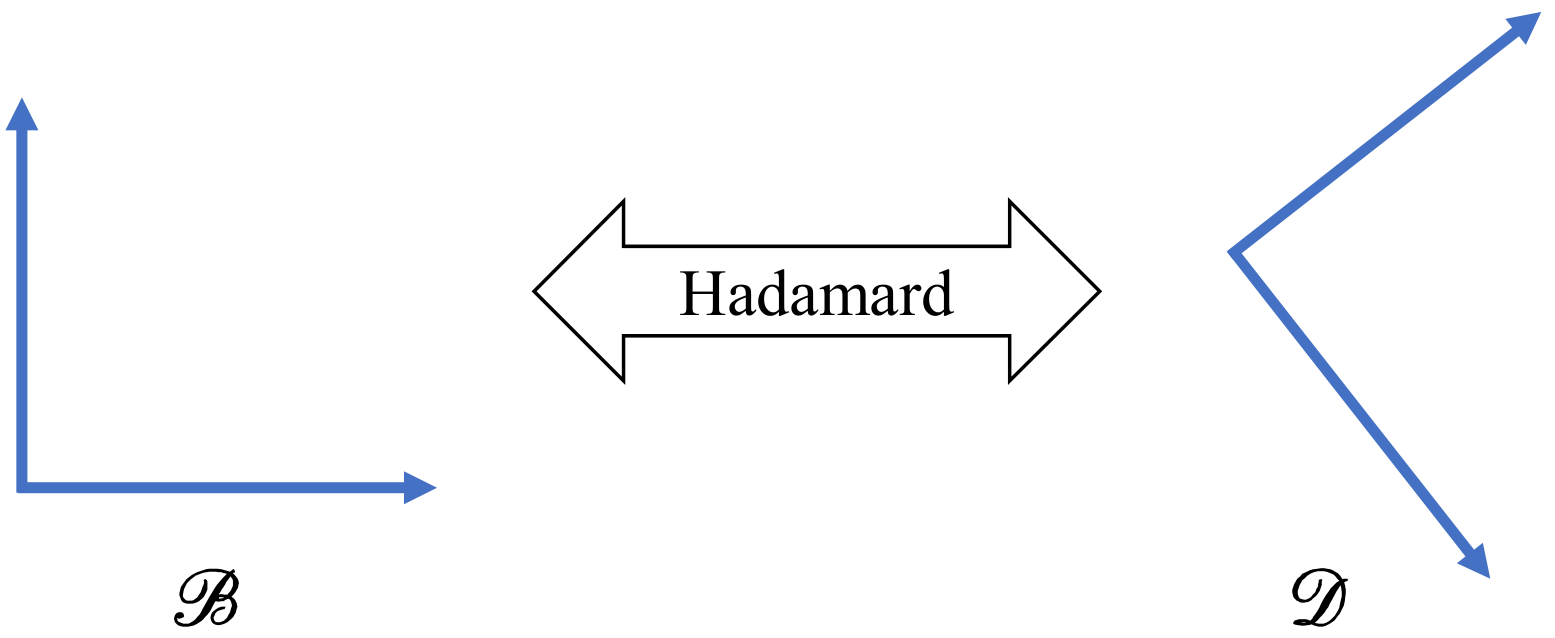
Figure 1.1: The Hardamard matrix for basis transition

example: hadamard matrix

ex:hadamard In $\mathbb{R}^2$, the transition matrix from the canonical basis $\begin{Bmatrix} \begin{bmatrix} 1 \\ 0 \end{bmatrix}, \begin{bmatrix} 1 \\ 0 \end{bmatrix} \end{Bmatrix}$ to this other basis $\begin{Bmatrix} \begin{bmatrix} \frac{1}{\sqrt{2}} \\ \frac{1}{\sqrt{2}} \end{bmatrix}, \begin{bmatrix} \frac{1}{\sqrt{2}} \\ -\frac{1}{\sqrt{2}} \end{bmatrix} \end{Bmatrix}$ is the Hadamard matrix: $\mathbf{H}=\frac{1}{\sqrt{2}}\begin{bmatrix} 1& 1\\1& -1 \end{bmatrix} =\begin{bmatrix} \frac{1}{\sqrt{2}}& \frac{1}{\sqrt{2}}\\ \frac{1}{\sqrt{2}}& -\frac{1}{\sqrt{2}} \end{bmatrix}$ as shown in Figure 1.1.

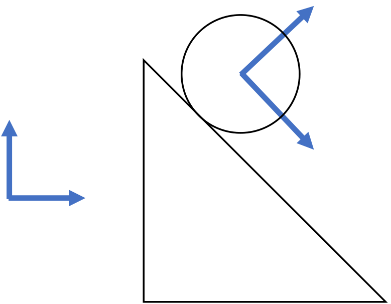
Figure 1.2: A ball rolling down a ramp

The motivation to change basis. In physics, we are often faced with a problem in which it is easier to calculate something in a noncanonical basis. For example, consider a ball rolling down a ramp as depicted in Figure 1.2.

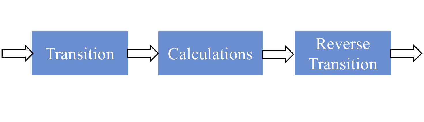
Figure 1.3: Problem-solving flowchart

The ball will not be moving in the direction of the canonical basis. Rather it will be rolling downward in the direction of +45◦, −45◦ basis. Suppose we wish to calculate when this ball will reach the bottom of the ramp or what is the speed of the ball. To do this, we change the problem from one in the canonical basis to one in the other basis. In this other basis, the motion is easier to deal with. Once we have completed the calculations, we change our results into the more understandable canonical basis and produce the desired answer. We might envision this as the flowchart shown in Figure1.3.

Throughout this course, we shall go from one basis to another basis, perform some calculations, and finally revert to the original basis. The Hadamard matrix will frequently be the means by which we change the basis.

Inner Product and Hilbert Space

Inner Product

definition

An inner product (also called a dot product or scalar product) on a complex vector space $\mathbb{V}$ is a function $\langle\cdot, \cdot\rangle:\mathbb{V}\times \mathbb{V}\rightarrow \mathbb{C}$ that satisfies the following conditions for all $\boldsymbol{v}$, $\boldsymbol{v}_1$, $\boldsymbol{v}_2$, and $\boldsymbol{v}_3$ in $\mathbb{V}$ and for $a, c\in \mathbb{C}$:

i. Nondegenerate: $\langle\boldsymbol{v}, \boldsymbol{v}\rangle\geq 0 \textrm{\ and\ } \langle\boldsymbol{v}, \boldsymbol{v}\rangle\Leftrightarrow \boldsymbol{v}=\boldsymbol{0}$

ii. Respects addition: $\begin{aligned} \langle\boldsymbol{v}_1+\boldsymbol{v}_2, \boldsymbol{v}_3\rangle&= \langle\boldsymbol{v}_1, \boldsymbol{v}_3\rangle + \langle\boldsymbol{v}_2, \boldsymbol{v}_3\rangle\\ \langle\boldsymbol{v}_1, \boldsymbol{v}_2+\boldsymbol{v}_3\rangle&= \langle\boldsymbol{v}_1, \boldsymbol{v}_2\rangle + \langle\boldsymbol{v}_1, \boldsymbol{v}_3\rangle \end{aligned}$

iii. Respects scalar multiplication: $\begin{aligned} \langle c\cdot \boldsymbol{v}_1, \boldsymbol{v}_2\rangle &= \overline{c}\times \langle \boldsymbol{v}_1, \boldsymbol{v}_2\rangle\\ \langle \boldsymbol{v}_1, c\cdot \boldsymbol{v}_2\rangle &= c\times \langle \boldsymbol{v}_1, \boldsymbol{v}_2\rangle \end{aligned}$ -->

iv. Skew symmetric: $\langle \boldsymbol{v}_1, \boldsymbol{v}_2\rangle = \overline{\langle \boldsymbol{v}_2, \boldsymbol{v}_1\rangle}$

definition

A vector space with an inner space.

example

The inner product is given as $\langle\boldsymbol{v}_1, \boldsymbol{v}_2\rangle=\boldsymbol{v}_1^{\top}\times \boldsymbol{v}_2$

example

ex:Cn $\mathbb{C}^n$: The inner product is given as $\langle\boldsymbol{v}_1, \boldsymbol{v}_2\rangle=\boldsymbol{v}_1^{\dagger}\times \boldsymbol{v}_2$

example

ex:Rnn $\mathbb{R}^{n\times n}$ has an inner product given for matrices $\mathbf{A}, \mathbf{B}\in\mathbb{R}^{n\times n}$ as $\langle\mathbf{A}, \mathbf{B}\rangle=\Tr(\mathbf{A}^{\top}\times \mathbf{B})$ where the trace of a square matrix $\mathbf{C}$ is given as the sum of the diagonal elements. That is, $\Tr(C)=\sum_{i=0}^{n-1}C[i,i]$

example

ex:Cnn $\mathbb{C}^{n\times n}$ has an inner product given for matrices $\mathbf{A}, \mathbf{B}\in\mathbb{C}^{n\times n}$ as $\langle\mathbf{A}, \mathbf{B}\rangle=\Tr(\mathbf{A}^{\dagger}\times \mathbf{B})$

definition

Norm is a unary function derived from inner product $|\cdot|: \mathbb{V}\rightarrow \mathbb{R}$ defined as $|\boldsymbol{v}|=\sqrt{\langle\boldsymbol{v},\boldsymbol{v}\rangle}$, which has the following properties

• Norm is nondegenerate: $|\boldsymbol{v}|>0 \textrm{\ if\ } \boldsymbol{v}\neq \boldsymbol{0} \textrm{\ and\ } |\boldsymbol{0}|=0$

• Norm satisfies the triangular inequality: $|\boldsymbol{v}+\boldsymbol{w}|\leq|\boldsymbol{v}|+|\boldsymbol{w}|$

• Norm respects scalar multiplication: $|c\cdot\boldsymbol{v}|=|c|\cdot|\boldsymbol{v}|$

definition

Distance is a binary function defined based on norm $d(\cdot, \cdot): \mathbb{V}\times \mathbb{V}\rightarrow \mathbb{R}$ defined as $d(\boldsymbol{v}_1, \boldsymbol{v}_2)=|\boldsymbol{v}_1-\boldsymbol{v}_2|=\sqrt{\langle\boldsymbol{v}_1-\boldsymbol{v}_2, \boldsymbol{v}_1-\boldsymbol{v}_2\rangle}$, which has the following properties

• Distance is nondegenerate: $d(\boldsymbol{v}, \boldsymbol{w})>0 \textrm{\ if\ } \boldsymbol{v}\neq\boldsymbol{w} \textrm{\ and\ } d(\boldsymbol{v}, \boldsymbol{w})=0\ \Leftrightarrow\ \boldsymbol{v}=\boldsymbol{w}$

• Distance satisfies the triangular inequality: $d(\boldsymbol{u}, \boldsymbol{v})\leq d(\boldsymbol{u}, \boldsymbol{w})+d(\boldsymbol{w}, \boldsymbol{v})$

• Distance is symmetric: $d(\boldsymbol{u}, \boldsymbol{v})=d(\boldsymbol{v}, \boldsymbol{u})$

definition

A basis $\mathcal{B}=\{\boldsymbol{v}_0, \boldsymbol{v}_1, \cdots, \boldsymbol{v}_{n-1}\}$ for an inner space $\langle\boldsymbol{v}_i, \boldsymbol{v}_j\rangle= \begin{cases} 1, & \textrm{if}\ \ i=j\\ 0, & \textrm{if}\ \ i\neq j \end{cases}$ with the following property

• For $\forall \boldsymbol{v}\in\mathbb{V}$ and any orthonormal basis $\{\boldsymbol{e}_i\}_{i=0}^{n-1}$ we have $\boldsymbol{v}=\sum_{i=0}^{n-1}\langle\boldsymbol{e}_i, \boldsymbol{v}\rangle\boldsymbol{e}_i$

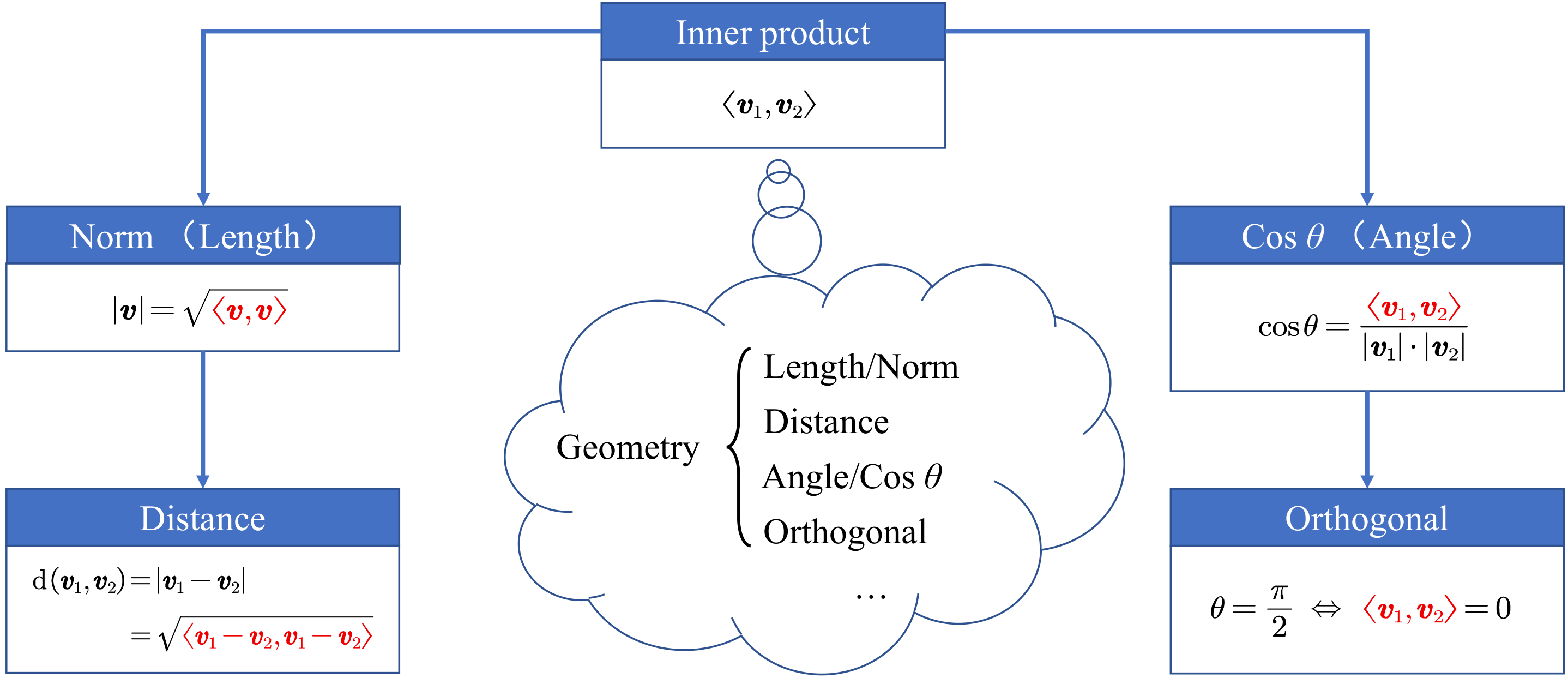
Note: inner product defines geometry in the vector space (Figure 1.4).

Figure 1.4: Inner product lays the geometric foundation in the vector space

Hilbert Space

definition

Within an inner product space $\mathbb{V}$, $\langle\cdot, \cdot\rangle$ (with the derived norm and a distance function), a sequence of vectors $\boldsymbol{v}_0, \boldsymbol{v}_1, \cdots$ is called a Cauchy sequence if $\forall \epsilon>0$, there exists an $N_0\in\mathbb{N}$ such that for all $m, n\geq N_0, d(\boldsymbol{v}_m, \boldsymbol{v}_n)\leq \epsilon$.

definition

For any Cauchy sequence $\boldsymbol{v}_0, \boldsymbol{v}_1, \cdots$, it is complete if there exist a $\overline{\boldsymbol{v}}\in\mathbb{V}$, such that $\lim\limits_{n\rightarrow \infty}d(\boldsymbol{v}_n-\overline{\boldsymbol{v}})=0$.

definition

A Hilbert space is a complex inner space that is complete.

Eigenvalue and Eigenvector

definition

For a matrix $\mathbf{A}\in\mathbb{C}^{n\times n}$, if there is a number $c\in\mathbb{C}$ and a vector $0\neq \boldsymbol{v}\in\mathbb{C}^n$ such that $\mathbf{A}\boldsymbol{v}=c\cdot\boldsymbol{v}$ then $c$ is called an eigenvalue of $\mathbf{A}$ and $\boldsymbol{v}$ is called an eigenvector of $\mathbf{A}$ associate with $c$.

Hermitian and Unitary Matrices

Hermitian Matrix

definition

An $n$-by-$n$ matrix $\mathbf{A}$ is called hermitian if $\mathbf{A}^{\dagger}=\mathbf{A}$. In other words, $A[j, k]=\overline{A[k, j]}$.

definition

If $\mathbf{A}$ is a hermitian matrix then the operator that it represents is called self-adjoint.

proposition

if $\mathbf{A}\in \mathbb{C}^{n\times n}$ is Hermitian, $\forall \boldsymbol{v},\boldsymbol{w}\in\mathbb{C}^{n}$ we have $\langle\mathbf{A}\boldsymbol{v}, \boldsymbol{w}\rangle=\langle\boldsymbol{v}, \mathbf{A}\boldsymbol{w}\rangle$

proof

Proof. $\begin{aligned} \langle\mathbf{A}\boldsymbol{v},\boldsymbol{w}\rangle &=\left(\mathbf{A}\boldsymbol{v}\right)^{\dagger}\times \boldsymbol{w} &\textrm{\textcolor{blue}{\ definition of inner product}}\\ &=\boldsymbol{v}^{\dagger}\times \mathbf{A}^{\dagger}\times \boldsymbol{w} &\textrm{\textcolor{blue}{\ multiplication relates to the adjoint}}\\ &=\boldsymbol{v}^{\dagger}\times \mathbf{A}\times \boldsymbol{w} \ &\textrm{\textcolor{blue}{\ definition of Hermitian matrices}}\\ &=\boldsymbol{v}^{\dagger}\times\left(\mathbf{A}\boldsymbol{w}\right) \ &\textrm{\textcolor{blue}{\ multiplication is associative}}\\ &=\langle\boldsymbol{v}, \mathbf{A}\boldsymbol{w}\rangle &\textrm{\textcolor{blue}{\ definition of inner product}} \end{aligned}$ ◻

:::

proposition

For a Hermitian matrix, its all eigenvalues are real.

proof

Proof. Let $\mathbf{A}\in\mathbb{C}^{n\times n}$ be a Hermitian matrix with an eigenvalue $c\in\mathbb{C}$ and an eigenvector $\boldsymbol{v}\in\mathbb{C}^n$ $\begin{aligned} c\langle\boldsymbol{v},\boldsymbol{v}\rangle &=\langle\boldsymbol{v}, c\boldsymbol{v}\rangle &\textrm{\textcolor{blue}{\ inner product respects scalar multiplication}}\\ &=\langle\boldsymbol{v}, \mathbf{A}\boldsymbol{v}\rangle &\textrm{\textcolor{blue}{\ definition of eigenvalue and eigenvector}}\\ &=\langle\mathbf{A}\boldsymbol{v}, \boldsymbol{v}\rangle &\textrm{\textcolor{blue}{\ see Proposition of Symmetry}}\\ &=\langle c\boldsymbol{v}, \boldsymbol{v}\rangle &\textrm{\textcolor{blue}{\ definition of eigenvalue and eigenvector}}\\ &=\overline{c}\langle\boldsymbol{v}, \boldsymbol{v}\rangle &\textrm{\textcolor{blue}{\ inner product respects scalar multiplication}}\\ \end{aligned}$ ◻

proposition

For a Hermitian matrix, distinct eigenvectors that have distinct eigenvalues are orthogonal

proof

Proof. Let $\mathbf{A}\in\mathbb{C}^{n\times n}$ be a Hermitian matrix with two distinct eigenvectors $\boldsymbol{v}_1\neq\boldsymbol{v}_2\in\mathbb{C}^n$ and their related eigenvalues $c_1,c_2\in\mathbb{C}$ $\begin{aligned} c_2\langle\boldsymbol{v}_1,\boldsymbol{v}_2\rangle &=\langle\boldsymbol{v}_1, c_2\boldsymbol{v}_2\rangle &\textrm{\textcolor{blue}{\ inner product respects scalar multiplication}}\\ &=\langle\boldsymbol{v}_1, \mathbf{A}\boldsymbol{v}_2\rangle &\textrm{\textcolor{blue}{\ definition of eigenvalue and eigenvector}}\\ &=\langle\mathbf{A}\boldsymbol{v}_1, \boldsymbol{v}_2\rangle &\textrm{\textcolor{blue}{\ see Proposition \ref{prop:symmetry}}}\\ &=\langle c_1\boldsymbol{v}_1, \boldsymbol{v}_2\rangle &\textrm{\textcolor{blue}{\ definition of eigenvalue and eigenvector}}\\ &=\overline{c_1}\langle\boldsymbol{v}_1, \boldsymbol{v}_2\rangle &\textrm{\textcolor{blue}{\ inner product respects scalar multiplication}}\\ &=c_1\langle\boldsymbol{v}_1, \boldsymbol{v}_2\rangle &\textrm{\textcolor{blue}{\ see proposition \ref{prop:real}}} \end{aligned}$ ◻

proposition

Every self-adjoint operator $\mathbf{A}$ on a finite-dimensional complex vector space $\mathbb{V}$ can be represented by a diagonal matrix whose diagonal entries are the eigenvalues of $\mathbf{A}$, and whose eigenvectors form an orthonormal basis for $\mathbb{V}$ (we shall call this basis an eigenbasis).

Physical Meaning of Hermitian Matrix. Hermitian matrices and their eigenbases will play a major role in our story. We shall see in the following lectures that associated with every physical observable of a quantum system there is a corresponding Hermitian matrix. Measurements of that observable always lead to a state that is represented by one of the eigenvectors of the associated Hermitian matrix.

Unitary Matrix

definition

Given a reversible matrix $\mathbf{U}\in\mathbb{C}^{n\times n}$ such that $\mathbf{U}\times \mathbf{U}^{\dagger} = \mathbf{U}^{\dagger}\times \mathbf{U}=\mathbf{I}_n$ then $\mathbf{U}$ is a unitary matrix.

example

$\mathbf{U}_1=\begin{bmatrix} \cos\theta &-\sin\theta &0\\[8pt] \sin\theta &\cos\theta &0\\[8pt] 0 &0 &1 \end{bmatrix}$ for any $\theta$. $\mathbf{U}_2=\begin{bmatrix} \frac{1+i}{2} &\frac{i}{\sqrt{3}} &\frac{3+i}{2\sqrt{15}}\\[8pt] \frac{-1}{2} &\frac{1}{\sqrt{3}} &\frac{4+3i}{2\sqrt{15}}\\[8pt] \frac{1}{2} &\frac{-i}{\sqrt{3}} &\frac{5i}{2\sqrt{15}} \end{bmatrix}$

proposition

If $\mathbf{U}\in\mathbb{C}^{n\times n}$ is unitary, $\forall \boldsymbol{v}, \boldsymbol{w}\in\mathbb{C}^n$ we have $\langle\mathbf{U}\boldsymbol{v}, \mathbf{U}\boldsymbol{w}\rangle=\langle\boldsymbol{v}, \boldsymbol{w}\rangle$

proof

Proof. Let $\mathbf{A}\in\mathbb{C}^{n\times n}$ be a Hermitian matrix with two distinct eigenvectors $\boldsymbol{v}_1\neq\boldsymbol{v}_2\in\mathbb{C}^n$ and their related eigenvalues $c_1,c_2\in\mathbb{C}$ $\begin{aligned} \langle\mathbf{U}\boldsymbol{v}, \mathbf{U}\boldsymbol{w}\rangle &=\left(\mathbf{U}\boldsymbol{v}\right)^{\dagger}\times \left(\mathbf{U}\boldsymbol{w}\right) &\textrm{\textcolor{blue}{\ definition for inner product}}\\ &=\boldsymbol{v}^{\dagger}\mathbf{U}^{\dagger}\times \mathbf{U}\boldsymbol{w} &\textrm{\textcolor{blue}{\ multiplication relates to adjoint}}\\ &=\boldsymbol{v}^{\dagger}\times \mathbf{I}\times \boldsymbol{w} &\textrm{\textcolor{blue}{\ definition for unitary matrices}}\\ &=\langle \boldsymbol{v}, \boldsymbol{w}\rangle &\textrm{\textcolor{blue}{\ definition for inner product}} \end{aligned}$ ◻

:::

proposition

If $\mathbf{U}\in\mathbb{C}^{n\times n}$ is unitary, $\forall \boldsymbol{v}, \in\mathbb{C}^n$ we have $|\mathbf{U}\boldsymbol{v}|=|\boldsymbol{v}|$

proof

Proof. Let $\mathbf{A}\in\mathbb{C}^{n\times n}$ be a Hermitian matrix with two distinct eigenvectors $\boldsymbol{v}_1\neq\boldsymbol{v}_2\in\mathbb{C}^n$ and their related eigenvalues $c_1,c_2\in\mathbb{C}$ $\begin{aligned} |\mathbf{U}\boldsymbol{v}| &=\sqrt{\langle\mathbf{U}\boldsymbol{v}, \langle\mathbf{U}\boldsymbol{v}\rangle} &\textrm{\textcolor{blue}{\ definition for norm}}\\ &=\sqrt{\langle\boldsymbol{v}, \boldsymbol{v}\rangle} &\textrm{\textcolor{blue}{\ unitary matrices preserve inner product}}\\ &=|\boldsymbol{v}| &\textrm{\textcolor{blue}{\ definition for norm}}\\ \end{aligned}$ ◻

:::

proposition

If $\mathbf{U}\in\mathbb{C}^{n\times n}$ is unitary, $\forall \boldsymbol{v}, \boldsymbol{w}\in\mathbb{C}^n$ we have $d(\mathbf{U}\boldsymbol{v}, \mathbf{U}\boldsymbol{w})=d(\boldsymbol{v}, \boldsymbol{w})$

proof

Proof. $\begin{aligned} d(\mathbf{U}\boldsymbol{v}, \mathbf{U}\boldsymbol{w}) &=|\mathbf{U}\boldsymbol{v}-\mathbf{U}\boldsymbol{w}| &\textrm{\textcolor{blue}{\ definition for distance}}\\ &=|\mathbf{U}(\boldsymbol{v}-\boldsymbol{w})| &\textrm{\textcolor{blue}{\ multiplication distributes over addition}}\\ &=|\boldsymbol{v}-\boldsymbol{w}| &\textrm{\textcolor{blue}{\ unitary matrices preserve norm}}\\ &=d(\boldsymbol{v}, \boldsymbol{w}) &\textrm{\textcolor{blue}{\ definition of distance}} \end{aligned}$ ◻

:::

proposition

The modulus of eigenvalues of unitary matrix is $1$.

proposition

Unitary matrix is the transition matrix from an orthonormal basis to another orthonormal basis.

Physical meaning of unitary Matrix. What does unitary really mean? As we saw, it means that it preserves the geometry. But it also means something else: If $\mathbf{U}$ is unitary and $\mathbf{U}\mathbf{V}=\mathbf{V}^{'}$, then we can easily form $\mathbf{U}^{\dagger}$ and multiply both sides of the equation by $\mathbf{U}^{\dagger}$ to get $\mathbf{U}^{\dagger}\mathbf{U}\mathbf{V}=\mathbf{U}^{\dagger}\mathbf{V}^{'}$ or $\mathbf{V}=\mathbf{U}^{\dagger}\mathbf{V}^{'}$. In other words, because $\mathbf{U}$ is unitary, there is a related matrix that can "undo" the action that $\mathbf{U}$ performs. $\mathbf{U}^{\dagger}$ takes the result of $\mathbf{U}$'s action and gets back the original vector. In the quantum world, all actions (that are not measurements) are "undoable" or "reversible" in such a manner.

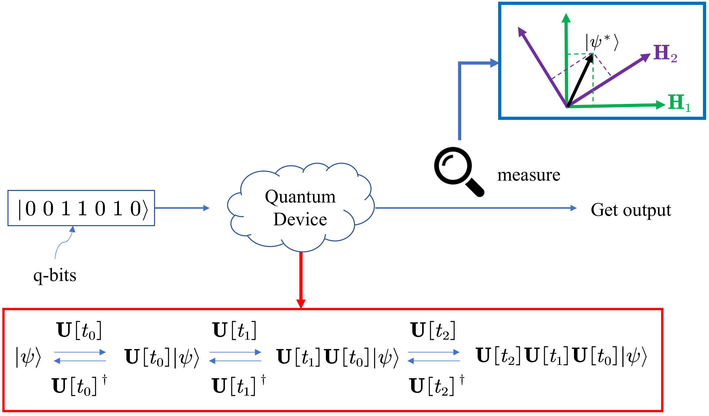
Figure 1.5: The role of Hermitian and unitary matrices

The roles of Hermitian and unitary matrices in quantum computing. As shown in Figure 1.5, the Hermitian matrix plays an important role in the quantum measurement phrase, which decides the concrete basis to observe the final computational result $\ket{\psi^{*}}$. Once the basis ($\mathbf{H}_1$ or $\mathbf{H}_2$) is decided, the observation result must be probabilistically collapsed into one of the eigenvectors of the corresponding basis. The unitary matrix plays a role of action to change the state of the quantum computer. 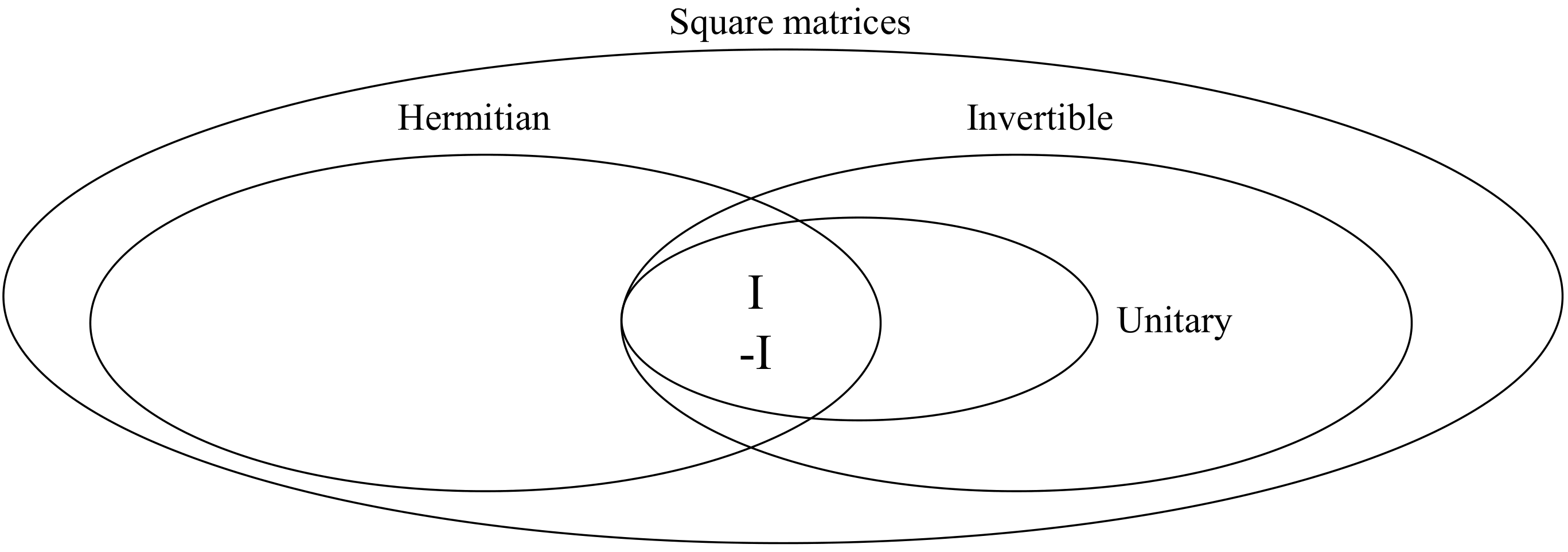Considering its reversible property, all actions performed in quantum computing can be undone by performing an action described by $\mathbf{U}^{\dagger}$. The relations of identity, Hermitian, unitary, and square matrices are shown in Figure 1.6.

Figure 1.6: Types of matrices.